
Tesseract OCR Introduction
Tesseract is considered one of the most accurate optical character recognition (OCR) engines. However, it fails to deliver satisfactory results in the case of noisy, low-quality images. So, even though the character recognition doesn’t seem that difficult from a human perspective, Tesseract sometimes needs assistance.
This article describes the steps we took to improve our Tesseract results with prior image processing in the context of a specific problem.
Problem Statement
As an input the program receives an image containing a single cell with a numeric value in the standard US price format:
- The value can be negative
- Starts with a dollar sign on the left
- Has a decimal point with two digits following on the right
- Has a comma after every third digit from right to left starting from the decimal point
The task is to recognize a numeric value and provide its string representation.


Testing of OCR
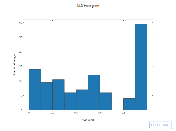
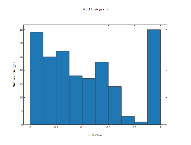
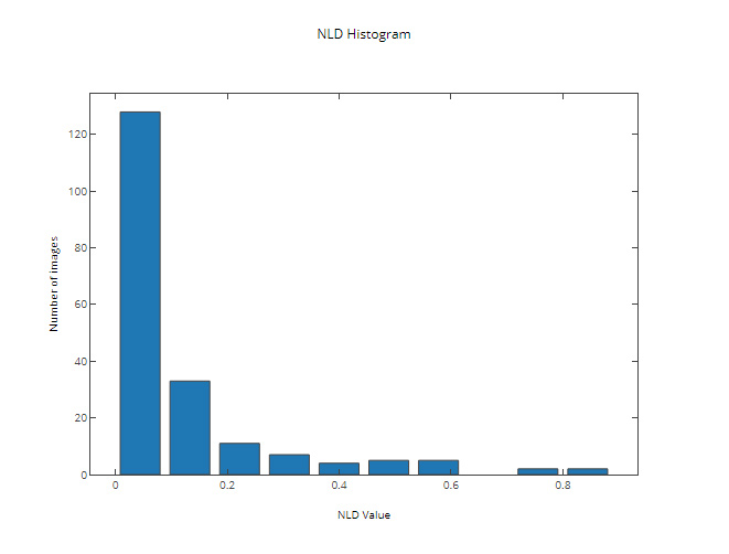
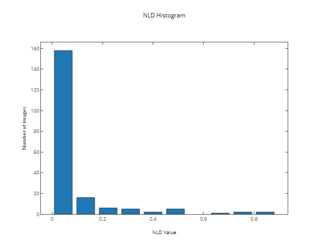
For testing, we used a set of nearly 200 images. At each step, we measured the percentage of correctly recognized images (which is our primary metric) and the distribution of NLD, where NLD is the normalized Levenshtein distance(1) between the recognized and the expected string. The NLD value is more descriptive and provides a better picture of the precision of the algorithm.
In a nutshell, the distribution of NLD value shows how close the recognized string is to the expected one, with the value 0.0 meaning an exact match and the value 1.0 meaning two completely different strings. Here are some examples of NLD:
    NLD("$1234.56", "") = 1.0
    NLD("$1234.56", "$") = 0.875
    NLD("$1234.56", "$1234.58") = 0.125
    NLD("$1234.56", "1$12341.56") = 0.2
    NLD("$1234.56", "$1234.56") = 0.0
Pure Tesseract results
Without any prior image processing, Tesseract was able to correctly recognize 14% of the test images with the following distribution of NLD:
The results on some of the test images:
| Input | Detected | Expected | NLD |
|---|---|---|---|
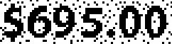
 |
$695.00 | 1.00 | |
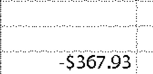 |
-$367.93 | 1.00 | |
 |
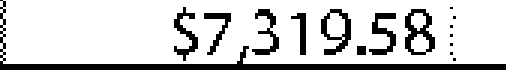
3,$319.58$ | $7,319.58 | 0.40 |
 |
$286.52 | 1.00 | |
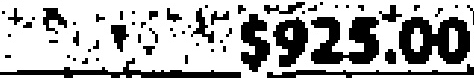 |
1$9,125.10 | $925.00 | 0.40 |
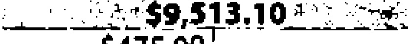 |
911.9-$-1- | $9,513.10 | 0.90 |
 |
$25.00 | 1.00 | |
 |
$13,591.40 | 1.00 | |
 |
$1,144.00 | 1.00 | |
 |
$22,297.30 | 1.00 | |
 |
$695.00 | 1.00 | |
 |
-$376.87 | 1.00 | |
 |
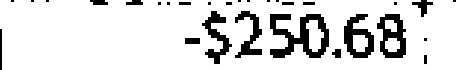
-1$2,506.37- | -$250.68 | 0.50 |
 |
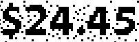
$24.45 | $24.45 | 0.00 |
 |
62,5-53,233,303,353,–$1–$-3–3.-1-3- | $7,302.62 | 0.89 |
 |
$1,989.53 | $198.00 | 0.44 |
 |
$68.30 | $68.00 | 0.17 |
 |
5,366.38 | $366.88 | 0.38 |
 |
$475.00 | $475.00 | 0.00 |
 |
$8,353.18 | $8,953.78 | 0.22 |
 |
-$55,135.83 | -$5,518.58 | 0.55 |
 |
$7,680.00 | $7,680.00 | 0.00 |
 |
$1,388.37 | 1.00 |
At this stage, it becomes obvious that even though the recognition of all test images looks simple from human a perspective, Tesseract requires assistance to complete the task with the desired accuracy.
Step 1: Extracting a Price Field
The first step we took was to extract a price field from an image prior to using Tesseract. For extracting a price field, we would convert an image to binary, find the connected areas on it and extract the part of an image containing the biggest group of connected areas lying on the same horizontal line.
Even though this step didn’t give us enough of a change in the percentage of correctly recognized images (16%), the improvements in the distribution of NLD are noticeable:
The results on some of the test images (with the extracted fields located in the “Extracted” column):
| Input | Extracted | Detected | Expected | NLD |
|---|---|---|---|---|
 |
|
$695.00 | 1.00 | |
 |
|
$367.93 | -$367.93 | 0.12 |
 |
|
$7,319.58$ | $7,319.58 | 0.10 |
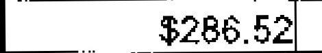
 |
|
$266.-52 | $286.52 | 0.25 |
 |
|
$925.00 | 1.00 | |
 |
|
1$9,513.10$ | $9,513.10 | 0.18 |
 |
|
$2,513.01 | $25.00 | 0.44 |
 |
|
51,335,913,031,3-13.–31 | $13,591.40 | 0.75 |
 |
|
$11,444,003,-419.35 | $1,144.00 | 0.63 |
 |
|
$22,329,730,3$$15.31 | $22,297.30 | 0.55 |
 |
|
$6,950.05- | $695.00 | 0.40 |
 |
|
-$376.87 | -$376.87 | 0.00 |
 |
|
$2,505.32 | -$250.68 | 0.56 |
 |
|
$24.45 | 1.00 | |
 |
|
35,331,933.63- | $7,302.62 | 0.71 |
 |
|
$1,980.13 | $198.00 | 0.44 |
 |
|
$68.00 | $68.00 | 0.00 |
 |
|
5,366.38 | $366.88 | 0.38 |
 |
|
$475.00 | $475.00 | 0.00 |
 |
|
$8,353.18 | $8,953.78 | 0.22 |
 |
|
-$5,518.58$ | -$5,518.58 | 0.09 |
 |
|
-$7,680.00 | $7,680.00 | 0.10 |
 |
|
$1,388.37 | 1.00 |
Step 2: Filtering out the Noise
For the next step, we filtered out connected areas with insignificant height (noise) from the extracted field. Note that this step also removes a minus sign, a decimal point and the commas from an image. However, since the format of the numeric values is predefined, the decimal point and commas can be recovered, and a minus sign is simple to detect by checking the connected areas to the left from the first significant one. Besides, as the first significant area is always a dollar sign, we don’t need Tesseract to detect it and therefore can remove it from an image as well. In the end, Tesseract needs only to detect the digits.
This step allowed us to make significant improvements in both the percentage of correctly recognized images (up to 64%) and the distribution of NLD:
The results on some of the test images (with the filtered images located in the “Filtered” column):
| Input | Filtered | Detected | Expected | NLD |
|---|---|---|---|---|
 |
|
$695.30 | $695.00 | 0.14 |
 |
|
-$367.93 | -$367.93 | 0.00 |
 |
|
$73,319.58 | $7,319.58 | 0.10 |
 |
|
$236.52 | $286.52 | 0.14 |
 |
|
$925.00 | $925.00 | 0.00 |
 |
|
$9,513.10 | $9,513.10 | 0.00 |
 |
|
$25.00 | $25.00 | 0.00 |
 |
|
$13,591.43 | $13,591.40 | 0.10 |
 |
|
$1,144.00 | $1,144.00 | 0.00 |
 |
|
$222,913,053.31 | $22,297.30 | 0.60 |
 |
|
$695.00 | $695.00 | 0.00 |
 |
|
-$37.68 | -$376.87 | 0.38 |
 |
|
-$250.63 | -$250.68 | 0.12 |
 |
|
$21.15 | $24.45 | 0.33 |
 |
|
$7,302.62 | $7,302.62 | 0.00 |
 |
|
$2,980.33 | $198.00 | 0.56 |
 |
|
$58.00 | $68.00 | 0.17 |
 |
|
$366.88 | $366.88 | 0.00 |
 |
|
$475.00 | $475.00 | 0.00 |
 |
|
$8,953.18 | $8,953.78 | 0.11 |
 |
|
-$5,518.53 | -$5,518.58 | 0.10 |
 |
|
$7,680.00 | $7,680.00 | 0.00 |
 |
|
$1,388.37 | $1,388.37 | 0.00 |
Step 3: Morphological Closing
After analyzing the images from our test set, we noticed that some of them still had noise attached to connected areas associated with the numeric value digits. To filter out the noise, we applied morphological closing. The example below shows how it helps to smooth an image:
Before:

After:

This resulted in an increase of of correctly recognized images (up to 80%) with the following NLD distribution:
The results on some of the test images (with the final images located in the “Final” column):
| Input | Final | Detected | Expected | NLD |
|---|---|---|---|---|
 |
|
$695.00 | $695.00 | 0.00 |
 |
|
-$367.93 | -$367.93 | 0.00 |
 |
|
$7,319.58 | $7,319.58 | 0.00 |
 |
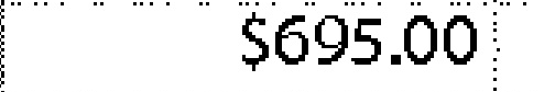
|
$286.52 | $286.52 | 0.00 |
 |
|
$925.00 | $925.00 | 0.00 |
 |
|
$9,513.10 | $9,513.10 | 0.00 |
 |
|
$25.00 | $25.00 | 0.00 |
 |
|
$135,914.03 | $13,591.40 | 0.45 |
 |
|
$1,144.00 | $1,144.00 | 0.00 |
 |
|
$222,973,013,121.31 | $22,297.30 | 0.63 |
 |
|
$695.00 | $695.00 | 0.00 |
 |
|
-$376.87 | -$376.87 | 0.00 |
 |
|
-$250.63 | -$250.68 | 0.12 |
 |
|
$24.45 | $24.45 | 0.00 |
 |
|
$7,302.62 | $7,302.62 | 0.00 |
 |
|
$198.00 | $198.00 | 0.00 |
 |
|
$68.00 | $68.00 | 0.00 |
 |
|
$366.83 | $366.88 | 0.14 |
 |
|
$475.00 | $475.00 | 0.00 |
 |
|
$8,953.78 | $8,953.78 | 0.00 |
 |
|
-$55,185.32 | -$5,518.58 | 0.45 |
 |
|
$7,680.00 | $7,680.00 | 0.00 |
 |
|
$1,388.37 | $1,388.37 | 0.00 |
Conclusion of Tesseract OCR usage
With prior image processing, we managed to increase the percentage of correctly recognized images from 14% to 80% and reduced the mean NLD value between the recognized and the expected string from 0.53 to 0.06.
References
- Normalized Levenshtein distance – Levenshtein distance divided by the maximum length of strings.
Authors: Anton Puhach, Michael Makarov
I can’t see a difference between the images in the columns input/extracted, input/filtered, input/final. Are the images correct?